Sometimes you may want to lock all or specific cells in an Excel 2016 worksheet to protect the date from being edited, altered or lost. Now, this post will show you how to do this.
Part 1: How to lock all cells in Excel 2016
Step 1: Open your worksheet in Excel 2016.
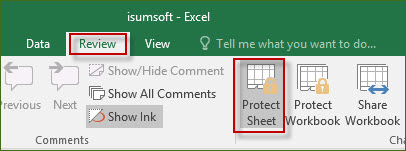
Step 2: Select the Review tab and then click on the Protect Sheet.

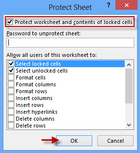
Step 3: In the Protect Sheet dialog, keep Protect worksheet and contents of locked cells checked, and then you can select how to protect the sheet and lock the cells, such as whether to assign a password to unprotect the sheet, whether to allow users to select locked/unlocked cells, whether to allow users to insert rows/columns, and so on. By default, it allows all users to select the locked and unlocked cells, but you can change this based on your own needs. After selecting what you allow users to do, click OK to confirm.

Then all the cells get locked as you required. To unlock the cells, just need to click on the Unprotect Sheet under the Review tab to unprotect the Excel worksheet 2016.
Part 2: How to lock specific cells in Excel 2016
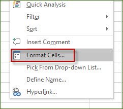
Step 1: On the Excel sheet, select the target cells you don’t want to lock. Right click on the selection and then select Format Cells from the menu.

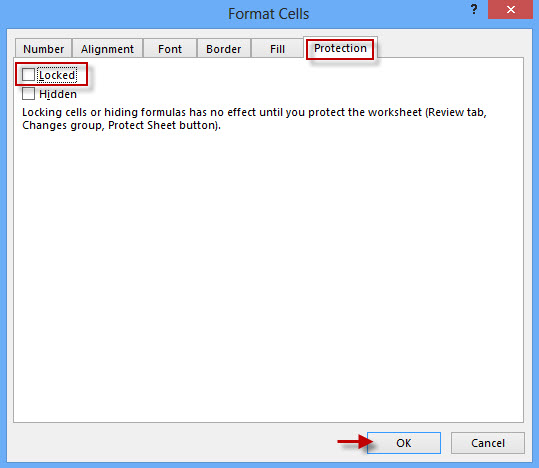
Step 2: After the Format Cells dialog opens, select the Protection tab, uncheck the box next to Locked, which is checked by default, and then click OK. This will unlock the selected cells. Unlocking will take effect after you protect the worksheet. So your next step is to protect the worksheet to unlock the selected cells and lock the rest of the cells.

Step 3: Select the Review tab, click on the Protect Sheet.
Step 4: In the Protect Sheet dialog, select what you want to allow all users of this worksheet to do, and click OK. This will lock the cells expect the specified cells you just selected in Step 1. To unlock them, you can still click on the Unprotect Sheet under the Review tab.

